QUADRATISING HAMILTON'S EQUATIONS
After some first initial developments (see this DAFx paper), Stefan and I have spent some effort attempting to improve the accuracy and the performance of the ``quadratised'' schemes. These are part of a new class of schemes of recent development, based on the idea of ``quadratisation'': when the nonlinear potential energy is non-negative, it can be written as the square of an auxiliary function. This leads to schemes for which the update is computable as the solution of a linear system, thus sidestepping the machinery of iterative root finders (these are needed for the update of classic fully-implicit schemes). Besides the obvious computational advantage, existence and uniqueness of the computed solution are proven by inspection of the update matrix alone. We wrote a couple of papers for the ENOC conference, held in Lyon, France, July 2022.

In the first one, we have a look at Hamiltonian systems, with the following Hamiltonian

Here, ψ = √2V, and the (nonlinear) potential is constrained such that V≥0. The resulting equations are

Above, the intermediate variable g=∇ψ has been introduced. Note that the Hamiltonian is composed of quadratic terms only (kinetic, linear potential and nonlinear potential energy components). Note as well that the auxiliary variable ψ is here a scalar: this kind of quadratisation is inherently different from the one that we have been using so far, e.g. for collisions, and for the nonlinear string (see also [1,2,3]).

A (VERY!) FAST ENERGY-CONSERVING INTEGRATOR
Integration of the above system may be performed as follows.

This scheme conserves a discrete energy-like quantity (sometimes called a pseudoenergy) [4]:

Note that the pseudoenergy is here of indefinite sign, as a consequence of the explicit discretisation of the linear part. However, the nonlinear energy is clearly non-negative, since it is proportional to ψ². Non-negativity of the energy can therefore be inferred from inspection of the linear part alone, leading to the following stability condition

This suffices to conclude that the scheme above is energy-stable. At a first glance, the scheme above looks implicit, and requiring the solution of a full linear system! On the surface, this looks considerably worse than the sparse update obtained with a vector ψ (like here). This is true, but here the update equation lends itself naturally to a fast inversion. Rewriting the terms above, one gets

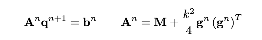
Here, Aⁿ, bⁿ are, respectively, a matrix and a vector of known coefficients. Aⁿ is in the form of a rank-1 perturbation to the diagonal mass matrix M, which can be inverted in O(N) operations using the Sherman-Morrison formula:

These schemes are really, really fast ... also, they can be applied to a vast class of problems, so long as the potential energy is bounded from below. Most problems in mechanics (and musical acoustics) are of this kind. One such system is the von Karman plate. Here, we managed to get compute times in Matlab of the same order as a fully explicit (but not energy-stable) scheme! This is pretty amazing ...

THE GEOMETRICALLY EXACT NONLINEAR STRING (AGAIN!)
In the second paper, we had a look at the geometrically exact nonlinear string. This is a long-time favourite ... You can read all about it here (see also [2,3,5]). As mentioned before, here we are performing a different kind of quadratisation with respect to our previous work: the auxiliary state function ψ is here a scalar, not a distributed quantity. We kind of went a bit further here, in that the model not only does it include the string, but also the hammer striking it (this is described by a highly nonlinear model, see here).
Here, the state vector is [u^T,v^T,U]^T, where u is the N×1 vector including the transverse displacements at the grid points; v is the N×1 vector of longitudinal displacements, and U is the displacement of the hammer. In continuous time, the equations of motion can be written as

where

and these are completed by the time derivative of ψ:

Here, M, C, K are, respectively, the (diagonal) mass matrix, the loss matrix (also diagonal), and the stiffness matrix, obtained from a finite difference spatial discretisation (but note that any other kind of discretisation would work too, like finite elements).
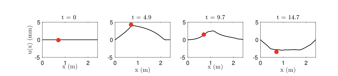
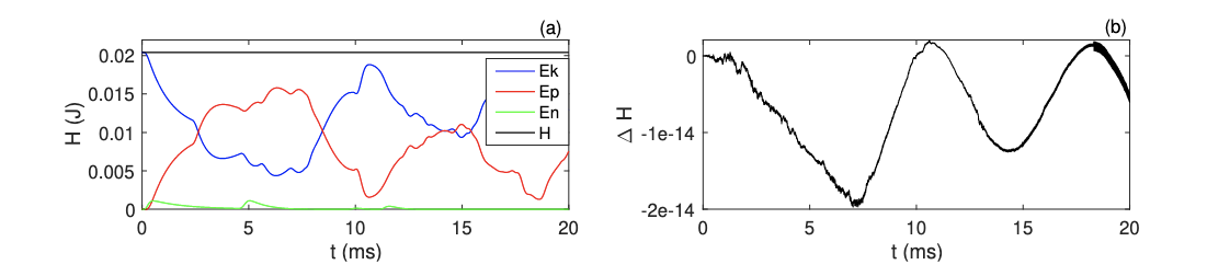
The interesting thing is that now all the nonlinearities are consolidated into the single scalar function ψ: these include the string inherent nonlinearity, and the hammer-string interaction. This is one reason why this method is so powerful: you can include pretty much anything in the definition of ψ, so long as the overall potential energy is non-negative. Here are some snapshot of the resulting dynamics

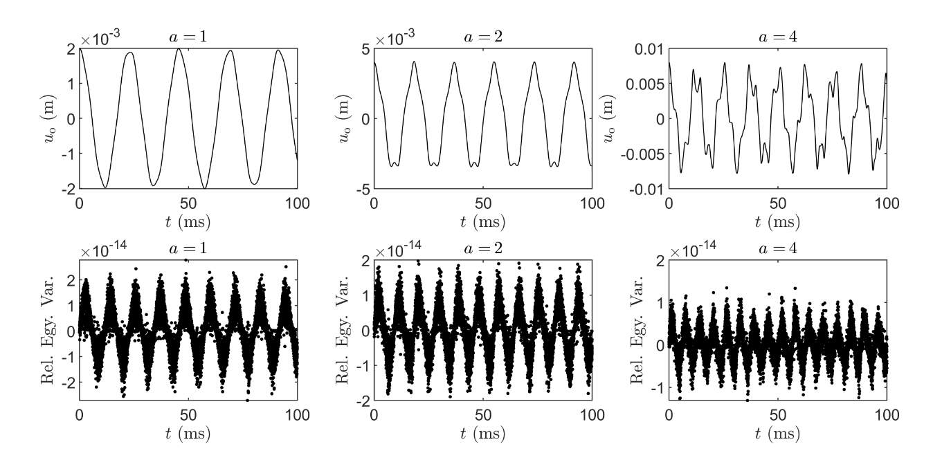
In the absence of losses, the scheme is conservative:

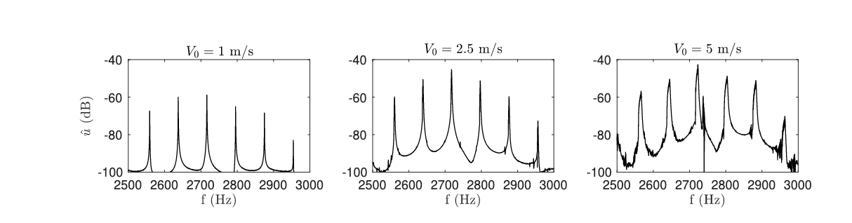
Here are some output spectra under various hammer's initial velocities. Note the change in brightness, as well as the appeareance of ``phantom partials''.

EXAMPLE SOUNDS
Here are example sounds. The grid spacing is chosen at the limit of stability of the longitudinal waves, so that h=k√E/ρ. This requires significant temporal oversampling, compared to audio rate. The sounds below are obtained using a sample rate of 12·48 kHz. What you are listening to below is the output velocity, taken at two output points along the string for stereo effect. The string parameters are taken from here. The examples below are a little too crude for realistic sound synthesis: most notably, there is no soundboard. However, the change in brightness and spectral content with increasing striking velocity is evident.

D2, V0= 1 m/s
D2, V0= 2.5 m/s
D2, V0= 5 m/s

D3, V0= 1 m/s
D3, V0= 2.5 m/s
D3, V0= 5 m/s

Here is a ``convergence'' test for the C2 string, using increasing values of the oversampling factor. An oversampling of at least 12 is usually needed for good resolution within the audio band, because of the large numerical dispersion in the transverse direction due to the choice of the large grid spacing.

C2, Oversampling factor (OF) = 8
C2, Oversampling factor (OF) = 12
C2, Oversampling factor (OF) = 16

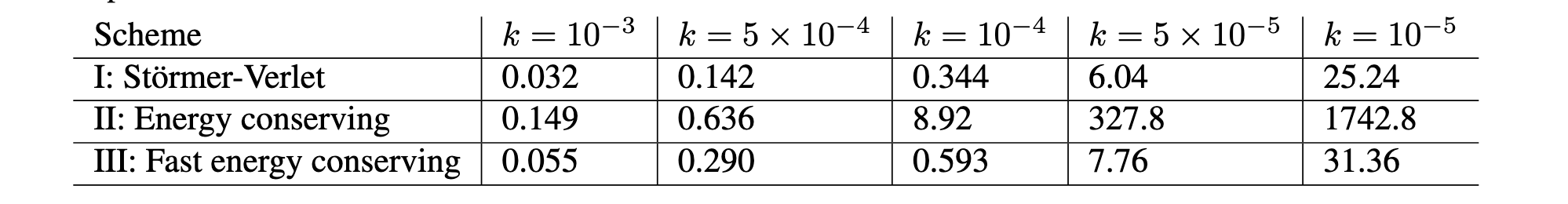
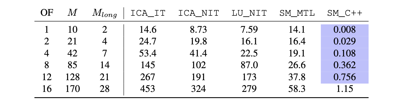
Finally, compute times. This is one of the most important results of this work: when coded properly in C++, the compute times for typical strings fall below real-time ... this is a huge accomplishment! Here, we are talking of systems with more than 200 nonlinearly coupled degrees of freedom. The speedup of the fast Sherman-Morrison scheme coded in C++, compared to a Matlab realisation of the iterative scheme, is around 350 times at OF = 12 ... this is absolutely huge!