THE GEOMETRICALLY EXACT NONLINEAR STRING
Nonlinear string vibration has been the subject of intense reasearch. Various musically relevant phenomena cannot be explained by linear theory alone: these include pitch glides and tension modulation effects. Geometric arguments and Hooke's law can be used to derive a nonlinear model, known in the literature as geometrically exact [1].

This model predicts an energy transfer (that is, a coupling) between the transverse and longitudinal waves. Numerically, this system is very complicated! (... and, from my perspective, a lot of fun to work with ...). Complications arise for two reasons. The first has to do with the linear parts of the longitudinal and transverse waves: these have very different wave speeds, ultimately impairing good numerical resolution. If you try to match the mesh size to either one of the wave speeds, you'll get severe warping in the other direction. The second difficulty arises as a consequence of classic time-stepping integrators, yielding an energy-conserving discretisation of the gradients on one hand, but a fully nonlinearly implicit discretisation on the other. This is a massive computational bottleneck!

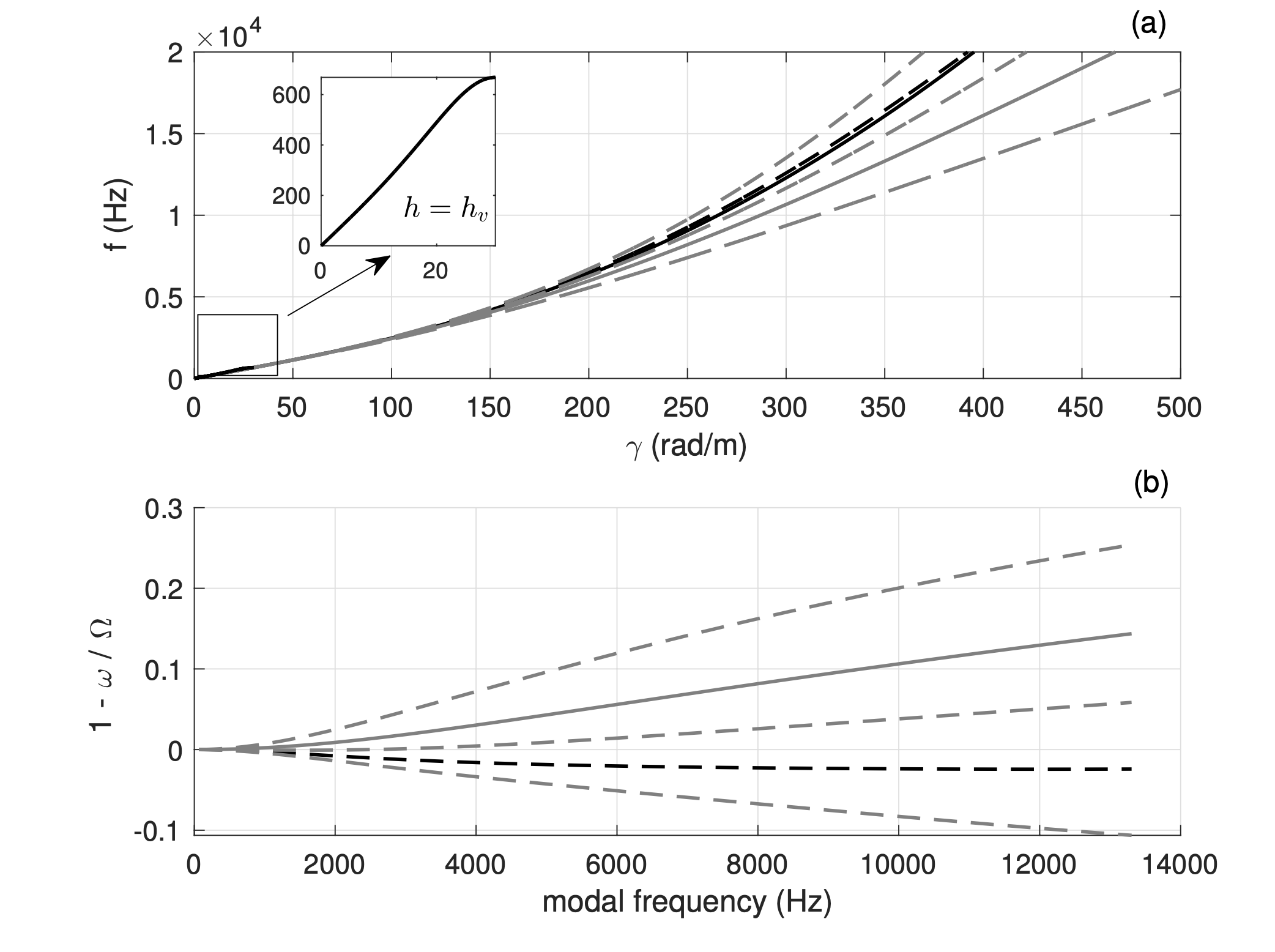
Stefan and I had a go with the problem. As a general design principle, it is always best to discretise the linear part as good as possible, that is, to make sure that the linear part runs with least amount of numerical dispersion possible with the sample rate available (for audio, say, 48 kHz or so). For the geometrically exact string, this takes a little tinkering, but we were able to discretise the transverse waves using a finite difference scheme, and the longitudinal waves using some kind of modal approach. Since, for audio, the sample rate (and hence, the time step), is used as input parameter, the grid spacing for the transverse difference scheme is chosen at the limit of stability, while the number of longitudinal modes can be selected so to match the number of actual eigenmodes of the continuous system, avoiding modal warping. The use of a free ``theta'' parameter, allows to match the numercal linear part of the transverse waves to the continuous model very, very closely.

CFL OR NOT?
The finite difference scheme for the transverse waves is characterised by a stability condition which depends on a switch η ∈ {0,1}. When η = 0, the fourth-order differential operator is discretised explicitly. This has consequences on the stability, convergence and accuracy properties of the scheme overall. When η = 0, k is not simply proportional to the grid spacing h. In fact, here k = O(h²), as opposed to a classic Courant–Friedrichs–Lewy (CFL) condition, obtained for η = 1, and which reads h = ck, where c is the wave speed. As a consequence, the formal order of accuracy in time of the scheme with η = 0 is only first-order! Is this scheme somewhat ``less accurate'' than a scheme with a pure CFL condition? This question can be addressed in a number of ways. Formal order-accuracy is of course one way of assessing the scheme's properties. But what happens if you look at the behaviour of the scheme in the frequency domain? Usually, in audio one selects the sample rate, and chooses the grid spacing at the limit of stability. So, if you compare the two schemes on this basis, the implicit scheme looks kind of clumsy in the frequency domain!

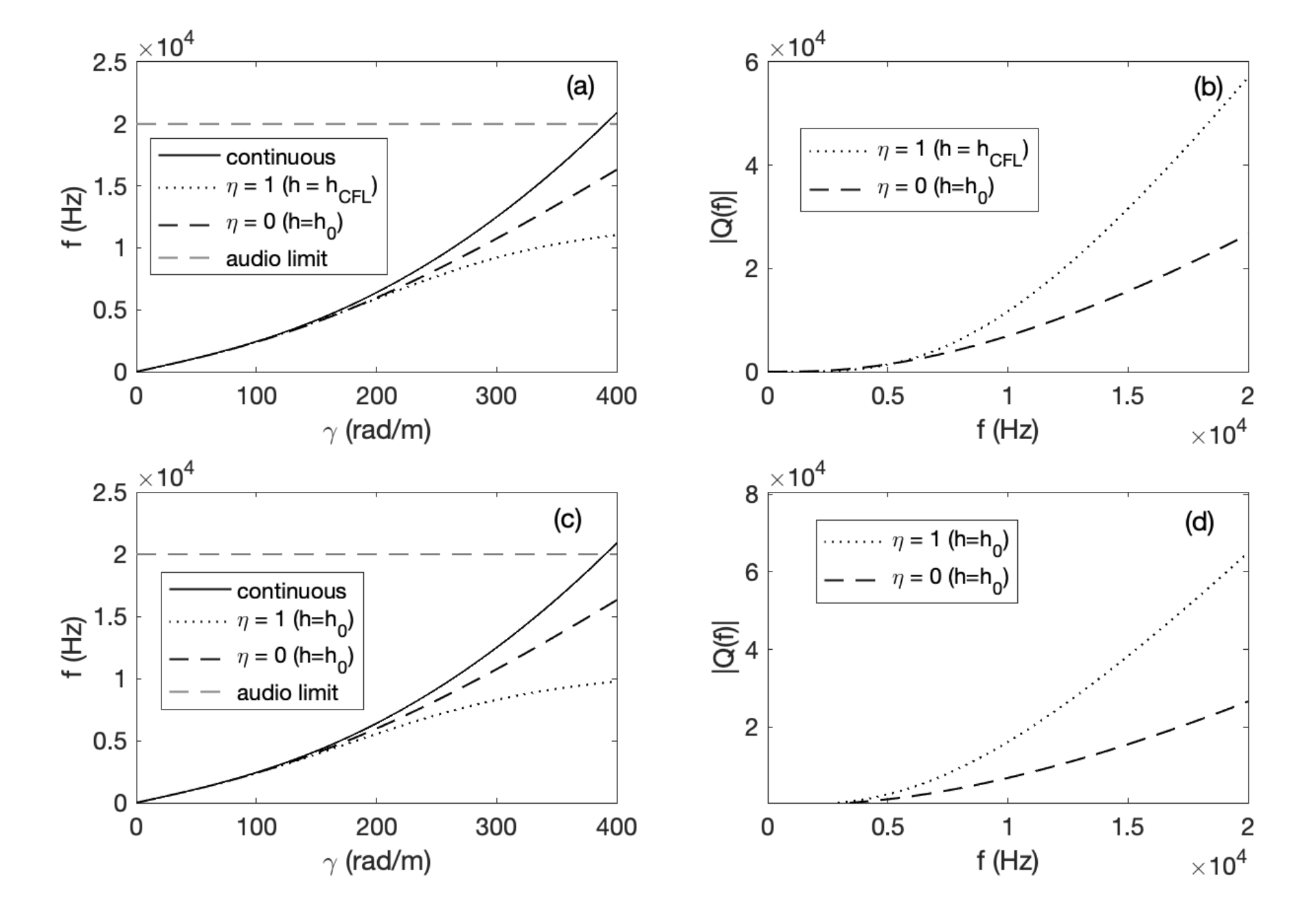
The figure above shows that the wideband properties of the schemes do not scale with order-accuracy. In other words, the scheme with η = 1 is way more accurate at lower frequencies, but numerical dispersion quickly gets worse at higher frequencies. For audio, this is not good, since a detuning of higher partials results in a string sounding ``flat''.
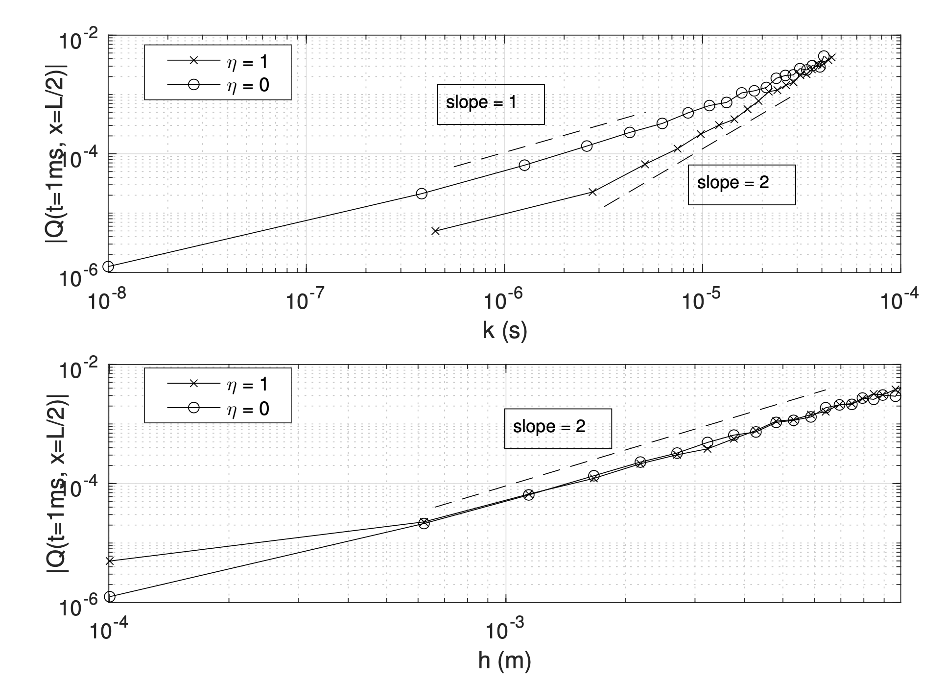
Okay, but what if you keep the grid spacing equal for both schemes, and select the time step at the limit of stability? Well, here the scheme with η = 0 clearly shows first-order accuracy ... but, for the same mesh size, the corresponding sample rate for this scheme is much larger, at the limit of stability, and this allows to compensate for the formal first-order accuracy ... in fact, when plotted against the mesh size h, the space-time errors for the two schemes are basically equal! Also, while the sample rate at the limit of stability is much lower for the scheme with η = 1, the scheme is η = 0 is nonetheless more efficient: the pentadiagonal system of the implicit scheme is a lot harder to do, than simple division ...

QUADRATISING THE NONLINEARITY
Now that the linear parts are sorted, we can have a look at the nonlinearity. As mentioned earlier, in classic time-stepping integrators, this is a real pain: on one hand, ensuring stability (that is, energy conservation) cannot be done using explicit designs. On the other hand, fully-implicit schemes result in huge algebraic nonlinear systems to be solved at each time step. This has a lot of side problems: you have to show existence and uniqueness of the numerical update; you need to decide on a nonlinear root finder (usually, Newton-Raphson), and you have to make choices regarding tolerance thresholds, halt conditions, ...

I have been investigating the possibility of alternative time-stepping discretisations, since my work on collisions [2]. The idea is really powerful: since potentials of interest in mechanics are often non-negative, you can map them onto a ``quadratised'' function. In practice, you define ψ = √2φ, and use ψ as an extra, indepedent state variable, to be solved for. Here's the magic: you are able to express update of this huge nonlinear system as a ... linear system! So, all you need really is one linear system solve at each time step. Existence and uniqueness are proven by simple inspection of the update matrix. Efficiency is obviously greatly improved. Here's what the time-stepping scheme looks like, from the article.

MATRIX DECOMPOSITION
The numerical scheme can be updated in a single pass, since the update equation looks like

In pratice, T is a block matrix, where the top left block is sparse, and is the largest (of size N X N), and where the bottom right is full, and is the smallest (of size N_s X N_s). Here N is the number of grid points for the transverse displacement, and N_s is the number of modal coordinates for the longitudinal component. Typically N_s≪N. In order to take advantadge of the sparsity of the upper left block, a block matrix LU decomposition can be employed. Details are given in the article. The proposed scheme, denoted LU_NIT, is compared to the two schemes given in [3]. The computational advantage of the current algorithm is pretty evident, especially compared to the fully-imlicit scheme.

EXAMPLE SOUNDS
Here are example sounds. For sound synthesis, loss and source terms are added. The simulations are run using this Matlab script. The scheme is pretty fast: at audio rate, for a string with ``average'' parameters, the compute time is less than 10 times real-time in Matlab.

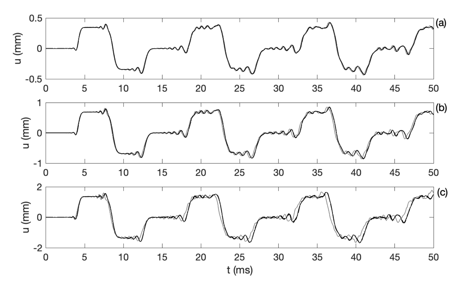
Here are some test cases. First, the string is picked with a small force (0.5 Newtons), and the output of the scheme at audio rate (48 kHz) and at 5X oversampling are compared. Here, I used ρ = 8000, L = 1.0, T₀ = 40, E = 2 · 10¹¹, and a radius r = 2.9 · 10^-4 (all units SI). The forcing acts at 0.72 L, and the forcing amplitudes are as indicated. Thanks to the novel discretisation, the scheme does not need to run at oversampled rates in this case. The two examples sound almost identical, as expected, since we took care of the linear part as good as we can with the available sample rate. The audio in the examples is postprocessed so that the velocity is recorded, not the displacement, at two output points along the string for stereo effect.

0.5 Newtons, 48 kHz
0.5 Newtons, 5X oversampling

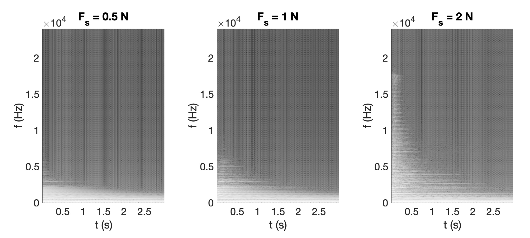
Then, the string is plucked with higher input forcings. The examples below are all run at audio rate (48 kHz), and compared to oversampled solutions. The scheme is able to capture all the most important aspects of nonlinear string vibration, even at audio rate, though a small oversampling factor may be needed for convergence (see figure below). Anyhow, this is a pretty good scheme. Maybe, with some extra work, we can approach real-time.

F = 1.0 N, 48 kHz
F = 1.0 N, 5X oversampling
F = 2.0 N, 48 kHz
F = 2.0 N, 5X oversampling

EXPERIMENTING WITH THE PHYSICS
You can get very interesting sounds using low pitched strings ... here, I used ρ = 12000, L = 1.5, T₀ = 40, E = 2 · 10¹¹, and a radius r = 2.9 · 10^-4 (all units SI). Force is again in the form of a raised cosine, with amplitude 2.5 and contact duration 0.0008, hitting at 0.72 L.

T0 = 40 N, 48 kHz
T0 = 20 N, 48 kHz

And here is again the string form the last example, but with different forcing parameters (maximum force F and contact duration t_w). You can really hear the phantom partials here ...

tw = 0.002 s, F = 2.5 N ,48 kHz
tw = 0.002 s, F = 0.5 N ,48 kHz

Experimenting with unrealistic parameters yields extremely interesting sounds ... Here's a beam with ρ = 12000, L = 3.5, T₀ = 20, E = 2 · 10¹¹, and a radius r = 4.9 · 10^-4. Forcing parameters are F = 4.5, t_w = 0.002 (all units SI). Sound designers out there, I am looking at you!

Long Beam,48 kHz

References

- J. Chabassier, P. Joly, Energy preserving schemes for nonlinear Hamiltonian systems of wave equations: Application to the vibrating piano string, Computer Methods in Applied Mechanics and Engineering, Vol. 199(45):2779–2795, 2010
- M. Ducceschi, S. Bilbao, S. Willemsen, S. Serafin, Linearly-implicit schemes for collisions in musical acoustics based on energy quadratisation, Journal of the Acoustical Society of America, Vol. 149(5):3502–3516, 2021
- M. Ducceschi, S. Bilbao. Non-iterative, conservative schemes for geometrically exact nonlinear string vibration, Proceedings of the International Congress on Acoustics (ICA2019), Aachen, Germany, 2019